
How To Add Pie Chart In Excel
How To Add Pie Chart In Excel - Quickly change a pie chart in your presentation, document, or spreadsheet. Change to a pie or bar of pie chart. You can format the labels to show specific labels elements like, the. To quickly identify a data series in a chart, you can add data labels to the data points of the chart. Learn best ways to select a range of data to create a chart, and how that data needs to be arranged for specific charts. To add text to a chart that is separate from the text in chart titles or labels, you can insert a text box on the chart. By default, the data labels are linked to values on the worksheet, and they update. For example, by adding a. In the spreadsheet that appears, replace the placeholder data with your own information. Visualize your data with a column, bar, pie, line, or scatter chart (or graph) in office. To use the alt text command on the quick access toolbar, select the shape, picture, chart, smartart graphic, or other object, click the toolbar button, and then add your alternative text. For example, by adding a. To quickly identify a data series in a chart, you can add data labels to the data points of the chart. Instead of entering text in the. By default, the data labels are linked to values on the worksheet, and they update. Change to a pie or bar of pie chart. For example, in the pie chart below, without the data labels it would be difficult to tell that coffee was 38% of total sales. Quickly change a pie chart in your presentation, document, or spreadsheet. Select insert > chart > pie and then pick the pie chart you want to add to your slide. The name of the chart) or axis titles (the titles shown on the x, y or z axis of a chart) and data labels (which provide further detail on a particular data point on. To quickly identify a data series in a chart, you can add data labels to the data points of the chart. Quickly change a pie chart in your presentation, document, or spreadsheet. Change to a pie or bar of pie chart. In the spreadsheet that appears, replace the placeholder data with your own information. For example, in the pie chart. Visualize your data with a column, bar, pie, line, or scatter chart (or graph) in office. Change to a pie or bar of pie chart. For example, in the pie chart below, without the data labels it would be difficult to tell that coffee was 38% of total sales. Select insert > chart > pie and then pick the pie. Select insert > chart > pie and then pick the pie chart you want to add to your slide. Using microsoft excel, you can quickly turn your data into a doughnut chart, and then use the new formatting features to make that doughnut chart easier to read. By default, the data labels are linked to values on the worksheet, and. Select insert > chart > pie and then pick the pie chart you want to add to your slide. Visualize your data with a column, bar, pie, line, or scatter chart (or graph) in office. Quickly change a pie chart in your presentation, document, or spreadsheet. To quickly identify a data series in a chart, you can add data labels. For example, by adding a. Change to a pie or bar of pie chart. Instead of entering text in the. Visualize your data with a column, bar, pie, line, or scatter chart (or graph) in office. Using microsoft excel, you can quickly turn your data into a doughnut chart, and then use the new formatting features to make that doughnut. Visualize your data with a column, bar, pie, line, or scatter chart (or graph) in office. For example, in the pie chart below, without the data labels it would be difficult to tell that coffee was 38% of total sales. By default, the data labels are linked to values on the worksheet, and they update. Select insert > chart >. Learn best ways to select a range of data to create a chart, and how that data needs to be arranged for specific charts. To use the alt text command on the quick access toolbar, select the shape, picture, chart, smartart graphic, or other object, click the toolbar button, and then add your alternative text. You can format the labels. You can then enter the text that you want. Instead of entering text in the. To quickly identify a data series in a chart, you can add data labels to the data points of the chart. Select insert > chart > pie and then pick the pie chart you want to add to your slide. For example, by adding a. Learn best ways to select a range of data to create a chart, and how that data needs to be arranged for specific charts. To use the alt text command on the quick access toolbar, select the shape, picture, chart, smartart graphic, or other object, click the toolbar button, and then add your alternative text. For example, in the pie. Visualize your data with a column, bar, pie, line, or scatter chart (or graph) in office. Select insert > chart > pie and then pick the pie chart you want to add to your slide. In the spreadsheet that appears, replace the placeholder data with your own information. To quickly identify a data series in a chart, you can add. The name of the chart) or axis titles (the titles shown on the x, y or z axis of a chart) and data labels (which provide further detail on a particular data point on. If your chart contains chart titles (ie. For example, by adding a. Change to a pie or bar of pie chart. To quickly identify a data series in a chart, you can add data labels to the data points of the chart. Learn how to create a chart in excel and add a trendline. To add text to a chart that is separate from the text in chart titles or labels, you can insert a text box on the chart. Explode the entire pie chart or just one piece. To use the alt text command on the quick access toolbar, select the shape, picture, chart, smartart graphic, or other object, click the toolbar button, and then add your alternative text. You can format the labels to show specific labels elements like, the. By default, the data labels are linked to values on the worksheet, and they update. You can then enter the text that you want. Quickly change a pie chart in your presentation, document, or spreadsheet. Instead of entering text in the. Visualize your data with a column, bar, pie, line, or scatter chart (or graph) in office. Select insert > chart > pie and then pick the pie chart you want to add to your slide.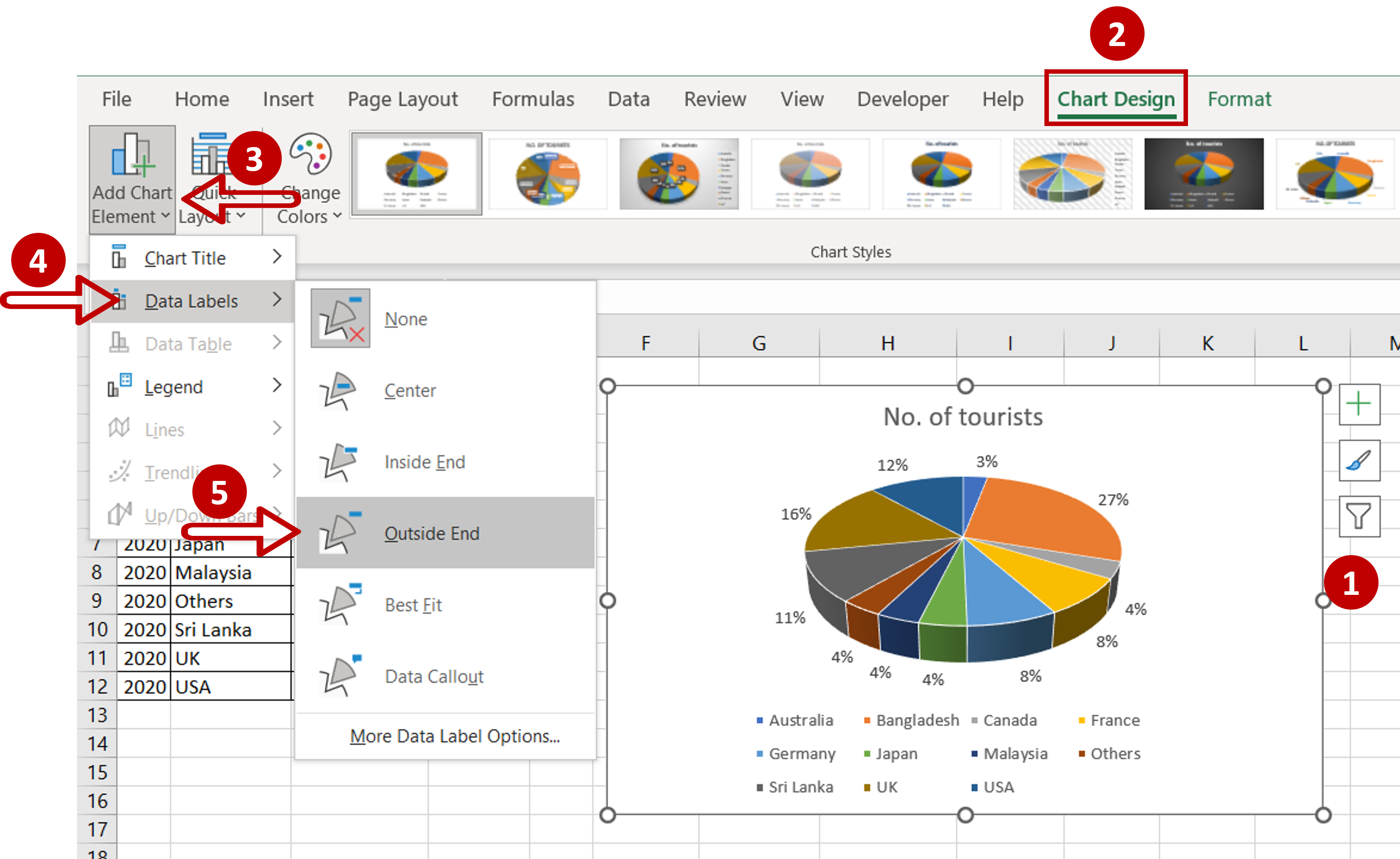
How To Insert A 3D Pie Chart In Excel SpreadCheaters
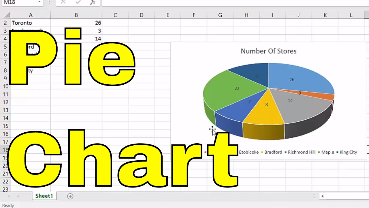
How To Create A Pie Chart In ExcelEASY Tutorial YouTube
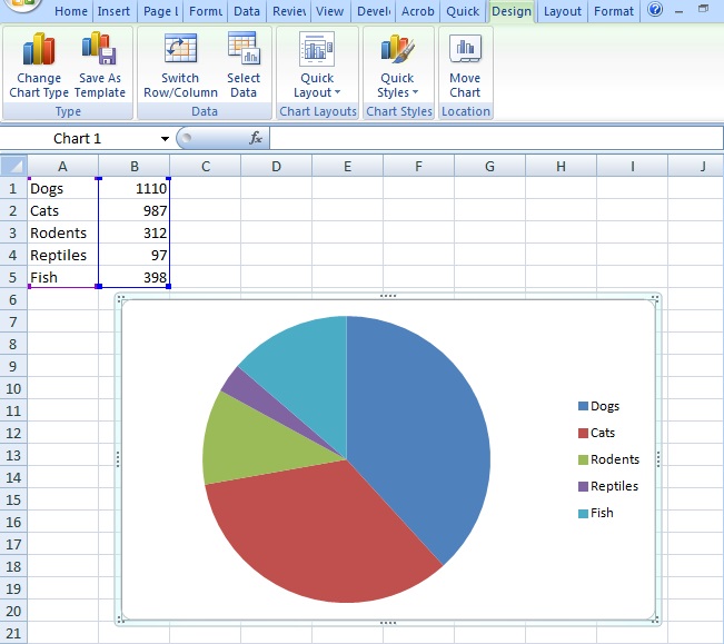
Pie Chart Definition, Examples, Make one in Excel/SPSS Statistics How To
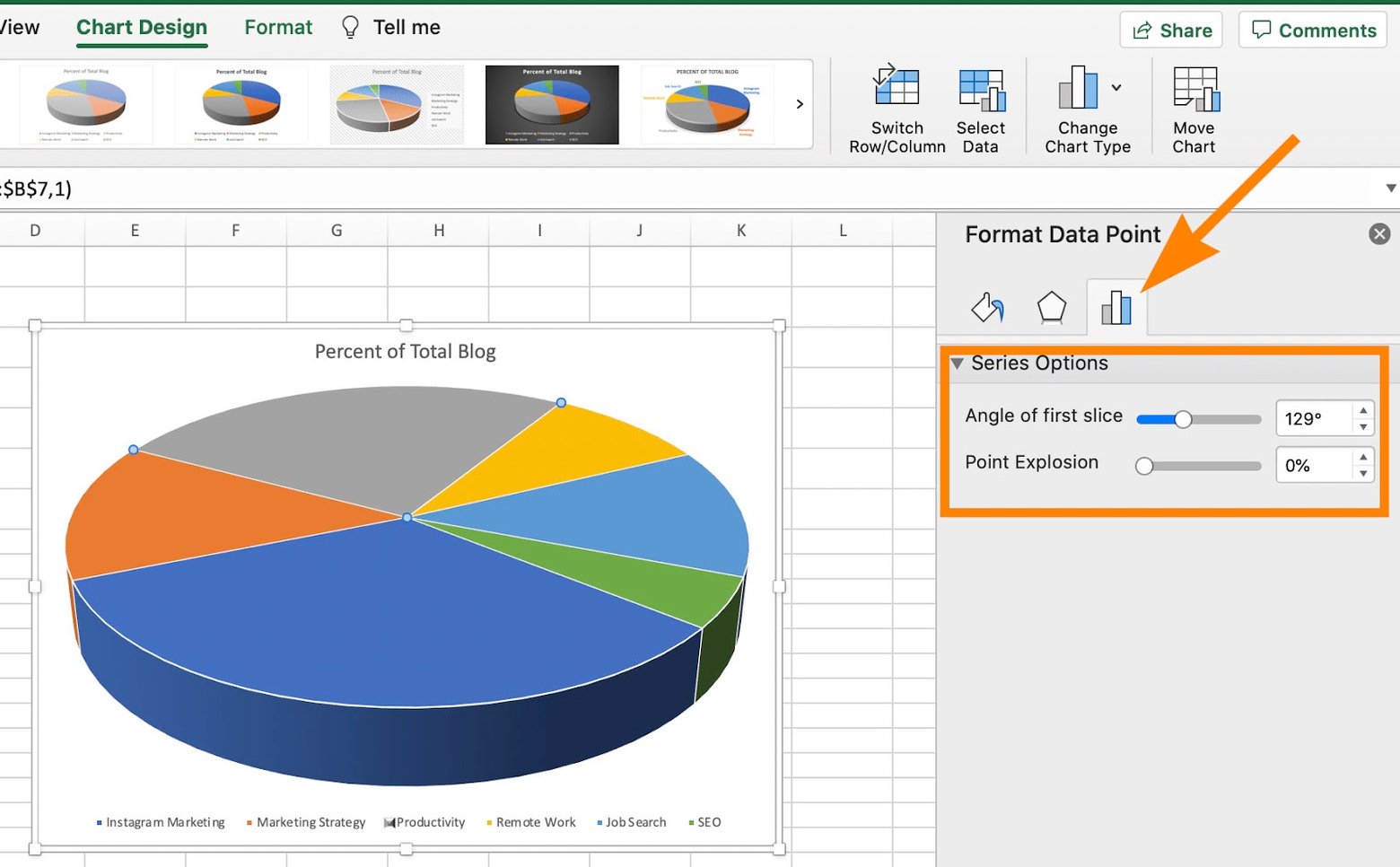
How to Create a Pie Chart in Excel in 60 Seconds or Less
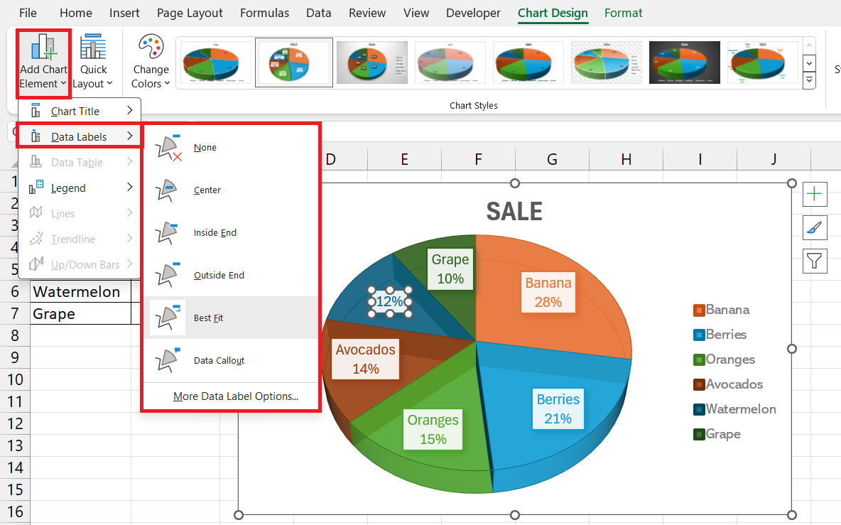
Create Pie Chart in Excel Like a Pro Fast & Simple Tutorial

How Do I Create A Pie Chart With Multiple Columns In Excel at Waldo Ross blog
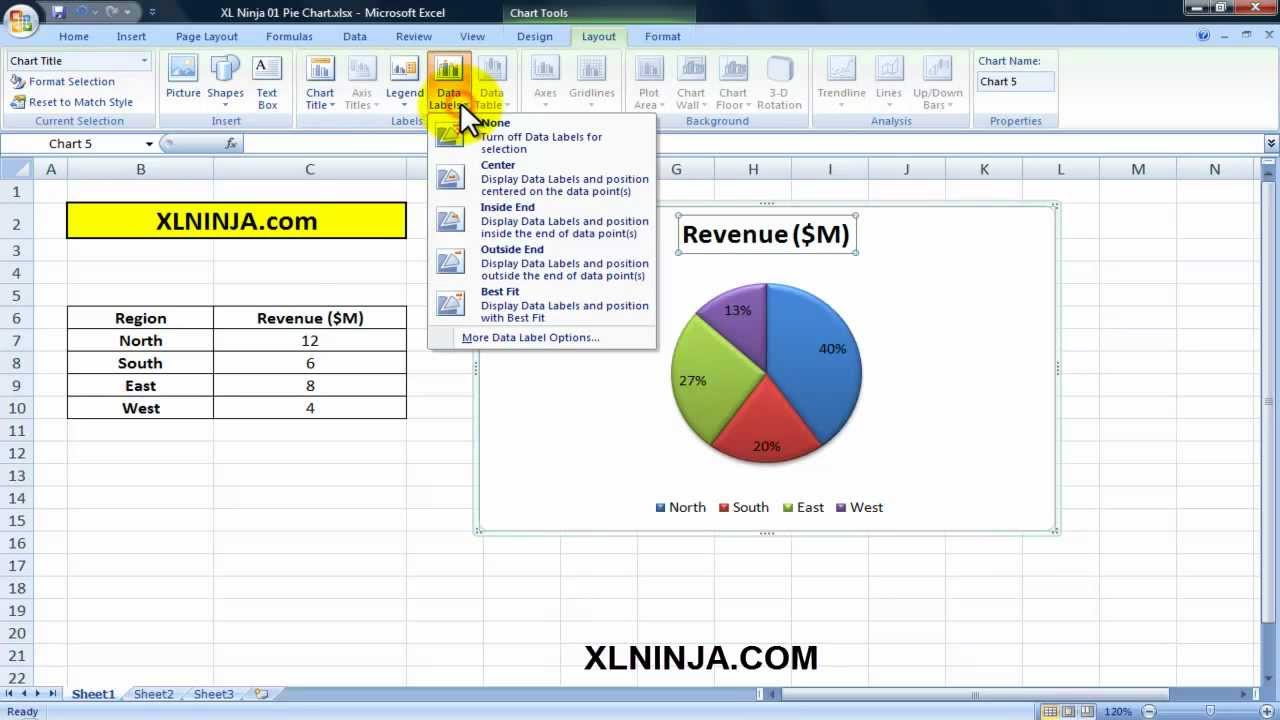
How To Add A Pie Chart To Excel Make A Pie Chart In Excel
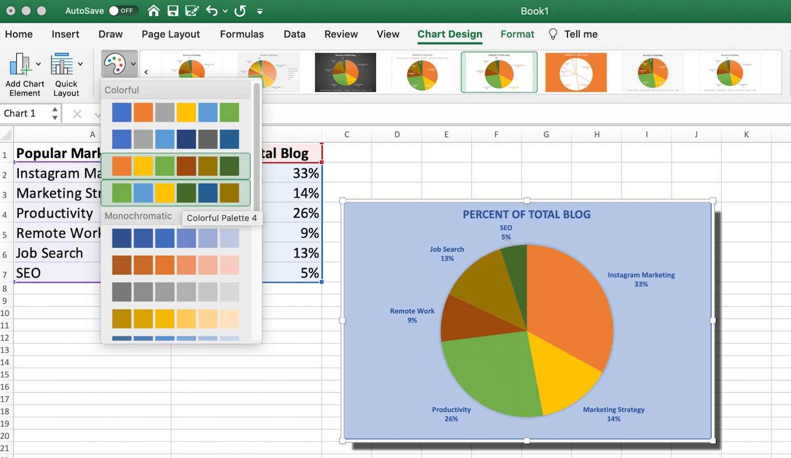
How to Create a Pie Chart in Excel in 60 Seconds or Less

How to Create a Bar of Pie Chart in Excel (With Example)
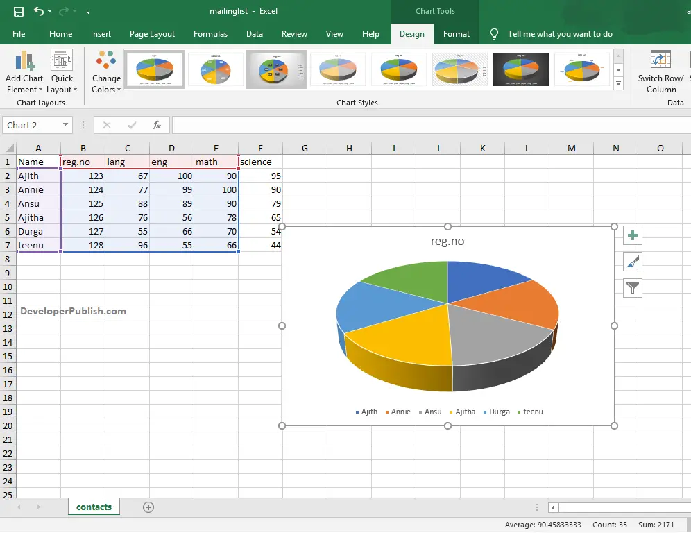
Pie Chart in Excel DeveloperPublish Excel Tutorials
In The Spreadsheet That Appears, Replace The Placeholder Data With Your Own Information.
Using Microsoft Excel, You Can Quickly Turn Your Data Into A Doughnut Chart, And Then Use The New Formatting Features To Make That Doughnut Chart Easier To Read.
For Example, In The Pie Chart Below, Without The Data Labels It Would Be Difficult To Tell That Coffee Was 38% Of Total Sales.
Learn Best Ways To Select A Range Of Data To Create A Chart, And How That Data Needs To Be Arranged For Specific Charts.
Related Post: